Has this ever happened to you? You have a storage device that fails at a customer site, but when you bring it in to engineering it passes all of your tests. You try to tailor your tests to closely simulate the customer environment, but just can't seem to duplicate the failure in your lab.

After all, a sequence of reads or writes is just a sequence of reads or writes.

Or is it?

Many times the difference between success and frustrating failure in these situations is in the details, and the purpose of this article is to look at a method of viewing those details.

As an example let's consider a disk subsystem. A customer application fails occasionally during random reads. Back in the lab your random read test runs with no problem. Let's look at what the difference in these random read situations really is.

This screenshot shows a trace capture of the failing application – note that it is just a series of 10 byte READ commands with random LBA addresses:

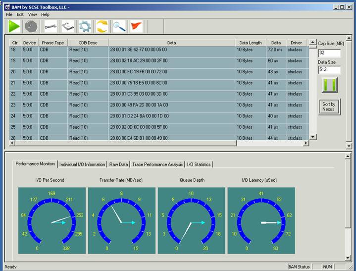
Just a series of random READ commands, but the beginning of the trace capture shown above tells several important things:

1. The application is using command tag queuing, and is achieving a queue depth of 16. This is shown by the series of READ commands with no data phases in between the commands, and is also shown on the Queue Depth gauge.
2. The data transfer size of the READ commands varies from command to command – this is seen more easily at the end of the capture, as shown below:

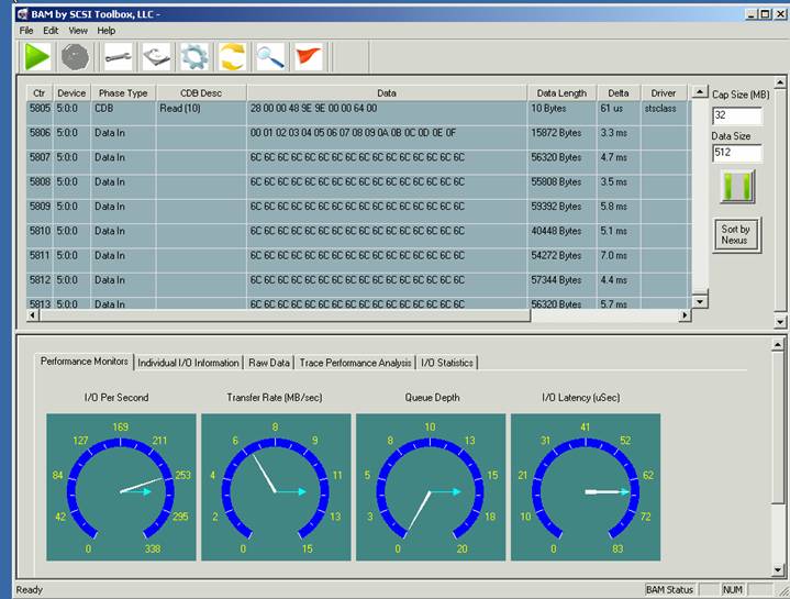
Here we see the queued data phases “catching up”. Note the different transfer sizes.

A few other important items to note are shown on the gauges – in particular take note of the I/O Latency. I/O latency is the amount of time in between commands – the lower the latency time the more commands can be issued in a given amount of time. A more detailed view of this parameter can be seen with the Trace Performance Analysis, as shown below:

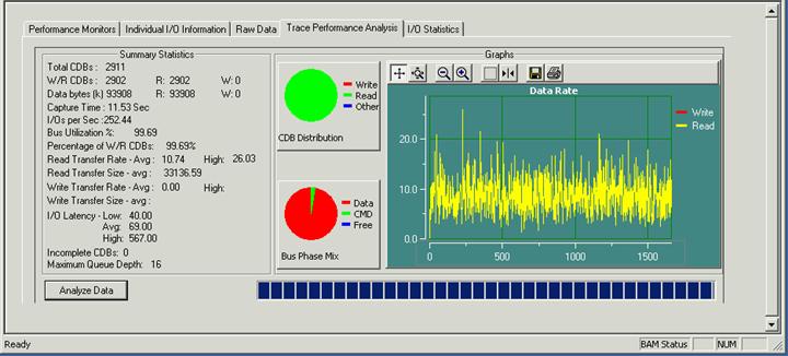
Note that over the course of the capture the I/O latency averaged 69 usec, with a low value of 40 usec. This allowed 252 I/O's per second to be issued.

Now let's have a look at our random read test used in our test lab. Here is a trace capture of this test running on the same drive as above:

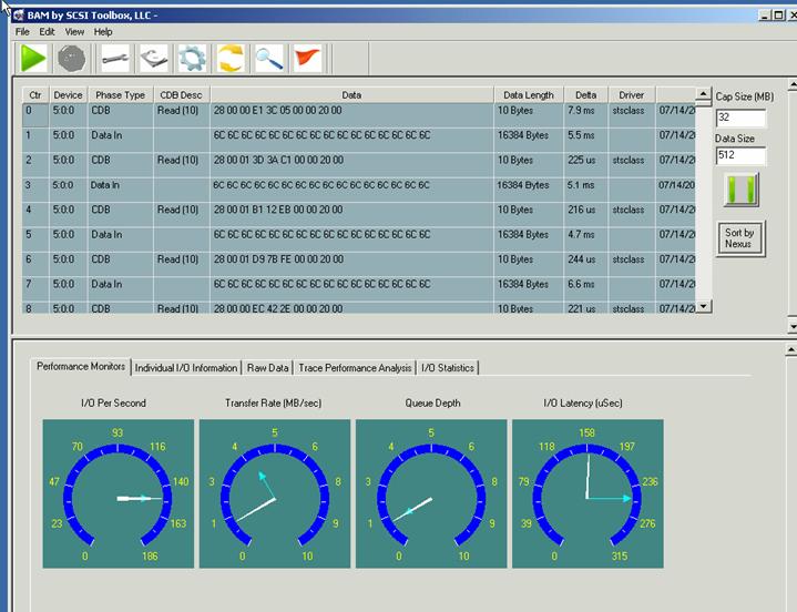
What stands out about our in-house test is:

1. The test is not using command tag queuing, as evidenced by the sequence of READ command, data, READ command, data, etc. The Queue Depth gauge confirms a queue depth of 1.
2. This test is issuing all of the READ commands with the same data size – in this case 16K per READ.
3. The I/O Latency is between 158 and about 250 usec. Let's have a look at the Trace Performance Analysis for a closer view:

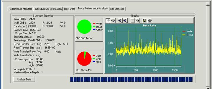
We now see that the I/O latency averaged 217 usec, with the lowest being 141 usec. This higher I/O latency time turns into a much lower number of I/O's per second – 147 versus 252.

The conclusion is that even though both situations are “just doing random reads” the two scenarios are very different, and the lab test is not stressing the disk system with as much data traffic as the failing application because the I/O rate is much lower, it is not using command tag queuing, and it is not varying the data transfer size.

In this case “just a random read test” is not just a random read test!

And the two lessons to be learned from this are:

1. Using the proper tools you can determine exactly what the parameters of a failure scenario are, and
2. It is important to tailor your lab tests to match the failing scenario as closely as possible.

Written by: Dr. SCSI